Quick Start

This walks you through your first measurement and the per-mode workflows. If a term is unfamiliar (NPLC, compliance, Enhanced R, etc.), see Concepts.

First measurement

1. Launch — resistamet-gui (or resistamet-gui --simulate for hands-free demo). On Windows with the .exe, double-click it.
2. Pick or create a user profile in the dialog that appears. Each user has their own settings and data directory.
3. Test connection — click the Test Connection button on any tab. Either:
   • In simulator mode, it should report a fake Keithley 2400 immediately.
   • With real hardware, it queries *IDN? and reports the detected model + firmware. If it fails, see Troubleshooting.
4. Enter a sample name at the top of the window — this names the CSV file written to disk.
5. Set source level and compliance on the active tab. Type natural units like 1mA, 5V, 100uA, 0.001 — the spinboxes accept engineering notation directly.
6. Click Start. Live readings appear, the plot updates in real time, the bottom strip shows V / I / R / P with their ± σ uncertainties.

What success looks like: The status bar reads Status: Running, the live readout has actual numbers (not --), and the plot fills in over time. If the readout shows 9.91e37 or stays at --, see Troubleshooting → Compliance hit / 9.91e37.

Per-mode workflows

For CSV schemas see Data Outputs; for parameter explanations see Concepts.

Resistance

Source a known current, measure resulting voltage, report R(t). Good for sensors, conductive composites, any DUT where you want resistance over time.

1. Choose 2-wire or 4-wire (4-wire eliminates lead resistance — preferred when possible).
2. Set Test current and Voltage compliance on the tab.
3. (Optional) Short the probes and click Null Cables to subtract lead resistance from every subsequent reading.
4. Click Start.

Enhanced accuracy is on by default (offset-compensated ohms, ~2× slower per reading, cancels thermoelectric EMF).

Voltage Source

Apply a DC voltage, monitor the resulting current. For chronoamperometry, device biasing, bias-stress experiments.

1. Set Source voltage, Current compliance, and Duration (0 = run until you click Stop).
2. Click Start.

A touch-safety warning fires before any run whose sourced voltage reaches the configured threshold (default 30 V).

Current Source

Mirror of Voltage Source — apply a DC current, monitor the resulting voltage. Same workflow with the source/measure roles swapped.

Four-Point Probe

Sheet resistance, resistivity, and conductivity via a collinear 4-point probe. ASTM F84-02 corrections applied automatically when you supply specimen geometry.

1. Set Source current, Probe spacing, and Thickness. Defaults: 100 µA, 0.1016 cm (Signatone SP4).
2. (Optional) Set specimen diameter, w/S, and temperature + dopant type to activate F₂ / F(w/S) / F_T corrections. Leaving these at defaults falls back to classical Smits-1958.
3. Click Start. Readings stream into the per-reading table; the live histogram fills in.
4. Click Save Spot to archive the current set. Move probe to next position and repeat.
5. Click Export Summary… for a per-spot + cross-spot CSV summary.

Probe power safety: default soft warn at 10 mW, hard stop at 100 mW (sized for tungsten-carbide SP4 tips). Pre-flight check refuses to start if worst-case I × V_compliance exceeds the hard stop.

Delta Mode (thermoelectric cancellation)

In the 4PP tab → Advanced → check Current Reversal (Delta Mode). Each reading then alternates +I / −I and reports V_delta = (V₊ − V₋) / 2.

Van der Pauw

ASTM F76-08 Method A for sheet resistance and resistivity on arbitrary-shape, hole-free samples with four periphery contacts.

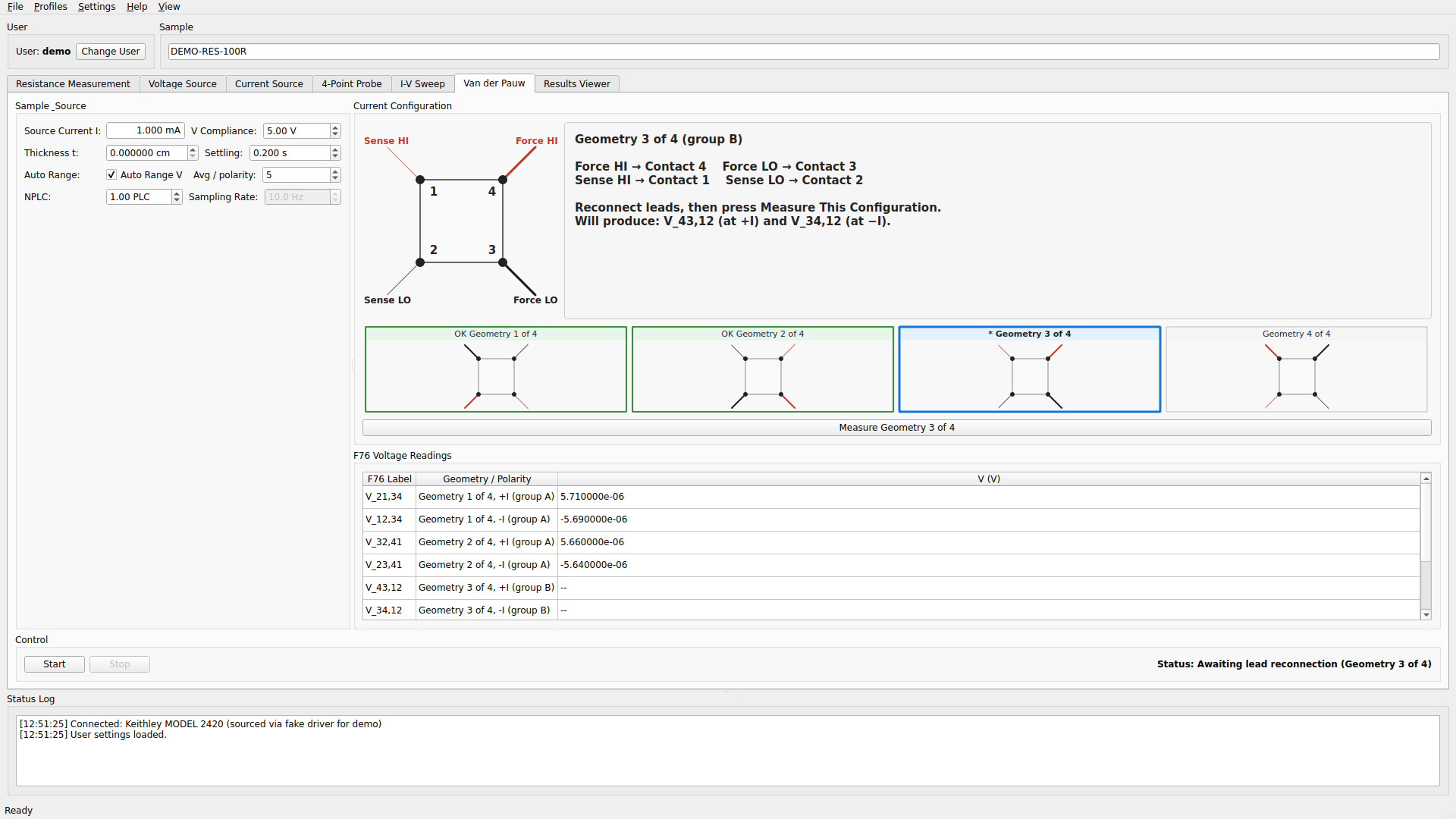
1. Number your four periphery contacts 1–4 counter-clockwise and connect leads.
2. Enter sample thickness in µm (required — you'll be prompted if you leave it blank).
3. Click Start. The tab shows a filmstrip of the four geometries. For each one: rewire your leads as shown in the sample diagram, then click Measure.
4. After all four geometries, the result panel reports sheet resistance, resistivity, F76 asymmetry, and a homogeneity pass/fail per F76 §11.1.

Output is disabled between geometries so you can safely reconnect leads.

I-V Sweep

Hardware staircase sweep using the Keithley's trigger model. Source voltage or current with configurable start, stop, step, and per-step delay.

1. Choose Source mode (V or I).
2. Set Start, Stop, Step, Per-step delay, and Direction (up, down, or up_down for hysteresis curves).
3. Click Start. The sweep runs on the instrument and the full I-V curve appears at the end.

Useful inputs

Type natural lab notation instead of raw decimals:

• 1mA instead of 0.001000 A
• 100uA or 100µA instead of 0.000100 A
• 10mV instead of 0.010 V

The live readout displays in engineering notation: V: 2.830 mV I: 1.000 mA R: 2.830 Ω with the Wong-palette label color per channel.

Other UI conveniences:

• Event markers — press M during a run; a dialog asks for a label (default MARK) which lands in the CSV's event column. The mark-event button on the active tab flashes yellow for 500 ms as visual confirmation.
• Tab keyboard shortcuts — Ctrl/Cmd + 1..6 jumps to tabs 1 through 6 (Resistance → vdP) without clicking
• Multi-user profiles — each user gets their own settings via the Settings → User Settings menu
• Parameter profiles — Profiles menu → Save / Load Profile for Current Mode writes/reads a JSON of the active tab's measurement-block settings (useful for per-sample-type templates)
• "Run until stopped" — set duration to 0 on timed modes for indefinite logging
• Tab switching during a run — the active tab keeps logging, inactive tabs are read-only; status bar shows "Viewing X tab (read-only) — Y measurement running"
• Smoothed live readout — the text readout updates at 4 Hz from a ~500 ms rolling mean over the last max(5, round(0.5 × sampling_rate)) samples, so noisy traces stay readable. The plot, CSV, and stats still see every full-rate sample.

Testing locally

# Unit + integration suite (sub-second)
QT_QPA_PLATFORM=offscreen pytest tests/ -v

# End-to-end suite (drives every tab through the in-package simulator,
# asserts recorded values against Ohm's law on a known fake DUT)
QT_QPA_PLATFORM=offscreen pytest tests/test_e2e_simulator.py -v

# Unit tests only (no Qt dependency)
pytest tests/ -v --ignore=tests/test_gui_smoke.py --ignore=tests/test_e2e_simulator.py

The e2e suite runs in its own pytest invocation because it leaves process-wide state (a pyvisa.ResourceManager monkey-patch and a live QApplication) that interacts poorly with module-scoped fixtures from earlier test files. CI runs both invocations in sequence.