Last week I was preparing a figure for a collaborator’s paper. I had a 100x SEM overview and a 5000x detail shot. I needed to draw a box on the overview showing where the detail came from.
I stared at both images for five minutes, trying to match features by eye. I guessed. The box was wrong.
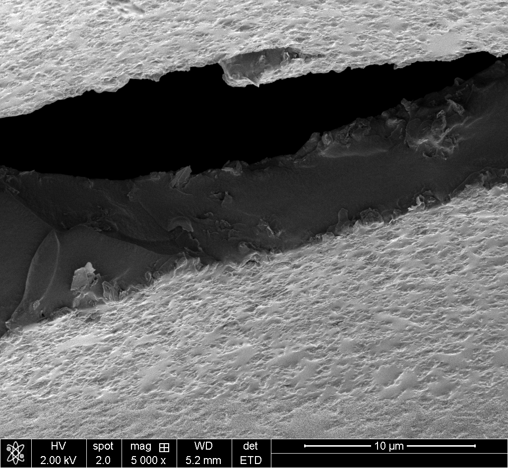
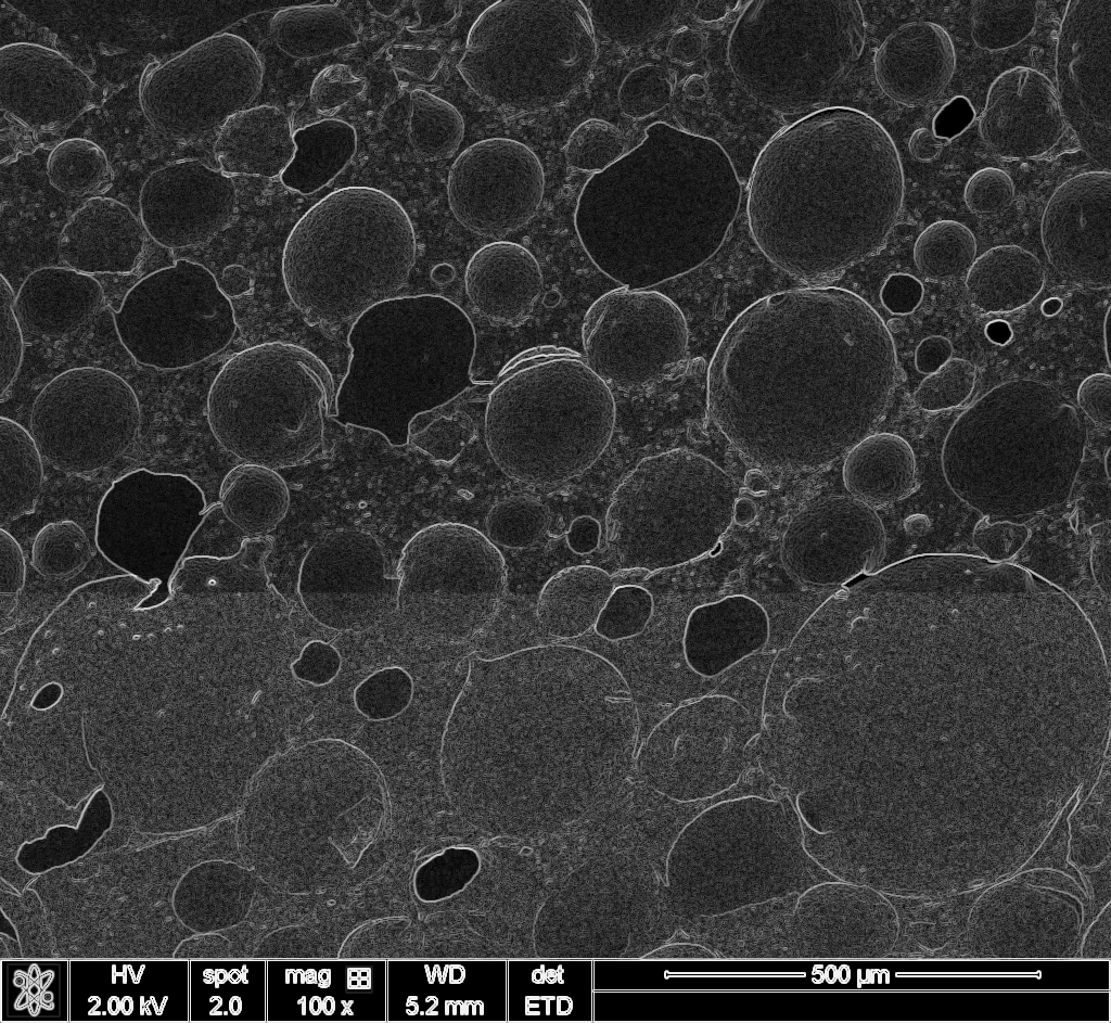
Try it yourself with some of my own polyHIPE foam images:

This happens constantly in microscopy. You zoom in on something interesting, capture it, then later need to show the spatial relationship between overview and detail. Manual annotation is tedious and error-prone. I wanted to automate it.
The idea
I knew template matching existed. I also knew that raw pixel matching wouldn’t work across a 50x magnification difference because the images look completely different at each scale. But edges persist. A pore boundary at 100x is still a boundary at 5000x, even if the textures are unrecognizable.
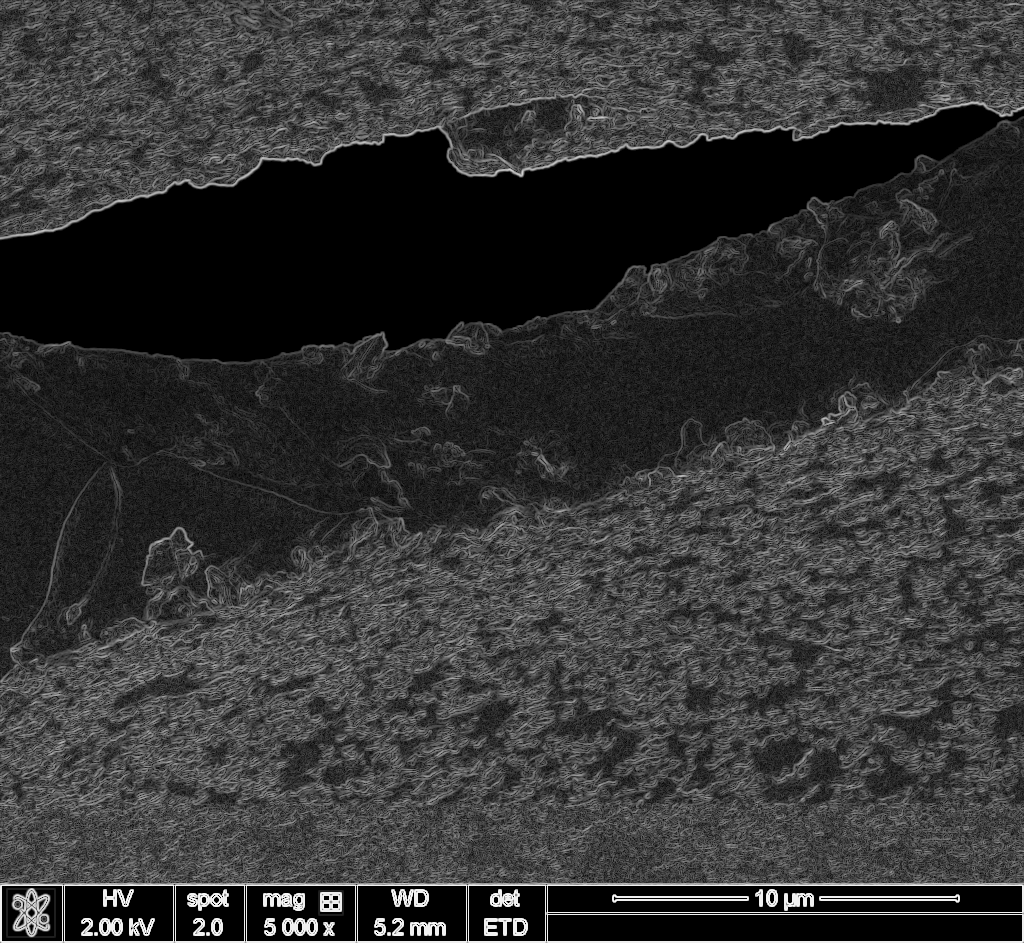
So my rough idea: compute edge maps for both images, then correlate them. Use FFT for speed.
I didn’t know how to implement this properly. I’m not a computer vision expert. But I had Claude Code.
The collaboration
I described the problem and my rough approach. Claude Code wrote the initial implementation: gradient magnitude via Sobel filters, FFT-based normalized cross-correlation, multi-scale search to find the optimal downsampling factor.
The first version worked on a simple test case. Then I threw the collaborator’s actual SEM images at it. The 5x and 10x ratio cases worked immediately. The 50x case (100x overview to 5000x detail) was harder. The detected region was just 26×22 pixels in the overview image.
Claude Code iterated on the visualization to make results clearer, added scale-vs-correlation plots to show the search process, and built a Colab notebook so I could share the tool.
Total time from “I have this annoying problem” to “here’s a working solution with documentation”: about ten minutes, including the five I spent staring at the images before giving up.
The results
The original images I was working with can’t be published (they belong to a collaborator), so I tested the tool on my own silicone polyHIPE SEM images. These are actually easier cases since there are fewer distinctive features competing for matches. The original images were more challenging.
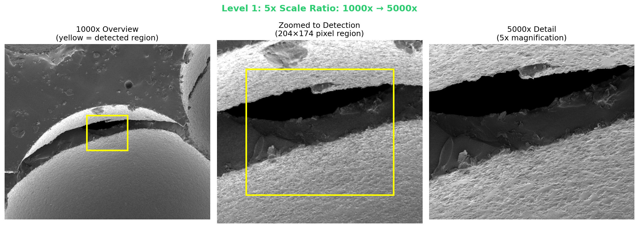
5x ratio (1000x → 5000x): Detected the 204×174 pixel region at exactly 5x scale.
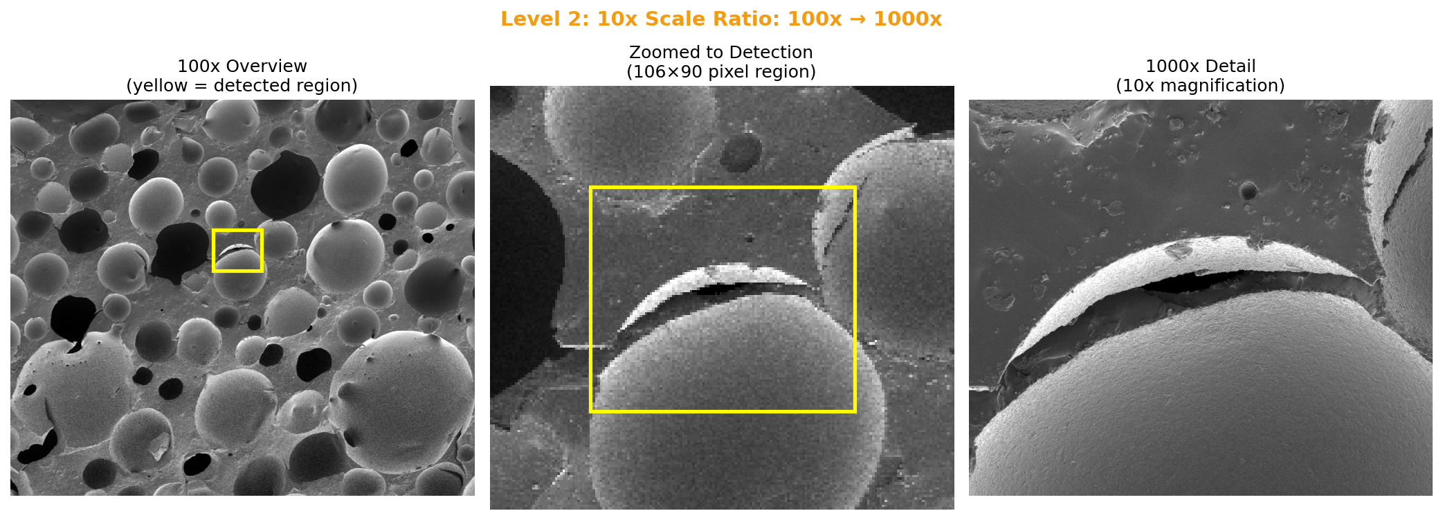
10x ratio (100x → 1000x): Found 9.6x scale (expected 10x). Region: 106×90 pixels.
50x ratio (100x → 5000x): This is the extreme case. Just 26×22 pixels in the overview. The algorithm found 40x (expected 50x), but the position was correct.
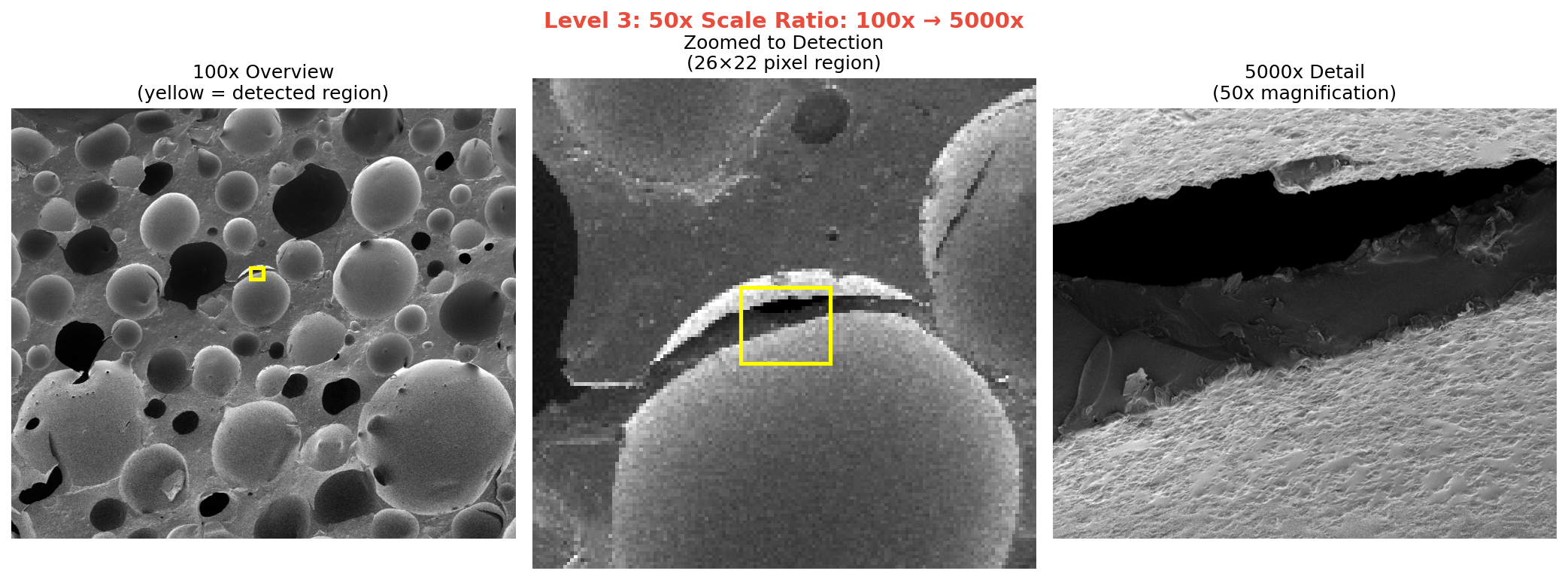
The correlation scores drop as scale ratio increases (0.059 → 0.020 → 0.0016), but that’s expected. At 50x magnification difference, the images share very little visual information. What matters is that the position is right.
The tool
I packaged this into a Google Colab notebook so anyone can use it. Upload an overview, upload a detail, set the expected scale range, run. It handles the preprocessing and produces a visualization showing where your detail image came from.
What I learned
I didn’t become a computer vision expert. I still couldn’t write this code from scratch. But I solved my problem, and now I have a reusable tool for future figures.
This is how I use Claude Code in my research: I bring domain knowledge (I know what SEM images look like, I know what problem I’m trying to solve, I have intuition about what approach might work) and Claude Code handles the implementation.